USAPhO 2012 A2
We’re gonna do another one of my favorites today: USAPhO 2012 A2!.
Solution
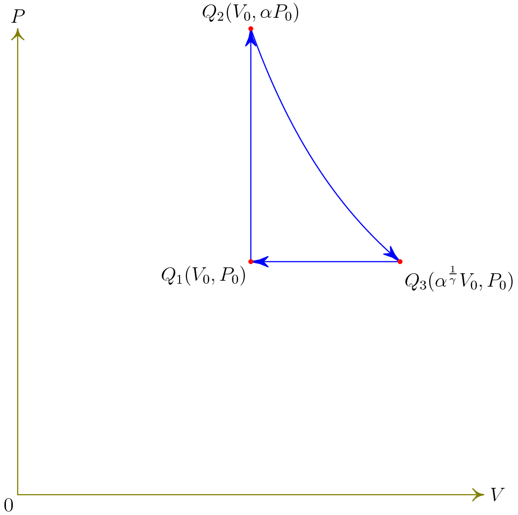
First we make a table and draw a P-V diagram, for educational purposes. I would not do either on an actual competition.
First, we start by finding missing values. Let us label the states through which the gas is taken through as 1, 2, 3, and 4, where 4 is equivalent to 1.
With some ease, we can say
| Index | $P$ | $V$ | $T$ |
|---|---|---|---|
| 1 | $P_0$ | $V_0$ | $T_0$ |
| 2 | $\alpha P_0$ | $ V_0 $ | $\alpha T_0$ |
| 3 | & | $P_0 V_0 \alpha^{\frac{1}{\gamma}}$ | $T_0 \alpha^{\frac{1}{\gamma}}$ |
| 4 | $P_0$ | $V_0$ | $T_0$ |
Here, we have use the ideal gas law and the adiabatic law that states $PV^{\gamma}$ is constant in an adiabatic process, where $\gamma = \frac{C_P}{C_V}$ is the adiabatic index.
Next, we make a P-V diagram. In case you wanted to screw around with it, the Asymptote code is provided.
[asy]
import graph;
unitsize(5cm);

int x = 2;
int y = 2;

draw((0, 0) -- (x, 0), arrow = ArcArrow(HookHead), olive);
draw((0, 0) -- (0, y), arrow = ArcArrow(HookHead), olive);

label("$V$", (x, 0), E);
label("$P$", (0, y), N);
label("$0$", (0, 0), SW);

real alpha = 2.0;
real gamma = 7.0/5.0;

real Vnaught = 1;
real Pnaught = 1;

draw((Vnaught, Pnaught) -- (Vnaught, Pnaughty * alpha), arrow = Arrow(HookHead), blue);
draw((Vnaught * alpha^(1.0/(gamma)), Pnaught) -- (Vnaught, Pnaught), arrow = Arrow(HookHead), blue);

real f(real x) {
return (Pnaught * (Vnaught^(gamma)) * alpha)/(x^(gamma));
}

path g = graph(f, Vnaught, Vnaught * alpha^((1.0/gamma)));
draw(g, arrow = Arrow(HookHead), blue);

dot((Vnaught, Pnaught), red);
dot((Vnaught, Pnaught * alpha), red);
dot((Vnaught * alpha^(1.0/(gamma)), Pnaught), red);

label("$Q_1 (V_0, P_0)$", (Vnaught, Pnaught), SW);
label("$Q_2 (V_0, \alpha P_0)$", (Vnaught, alpha * Pnaught), N);
label("$Q_3 (\alpha^{\frac{1}{\gamma}} V_0, P_0)$", (Vnaught * alpha^(1.0/(gamma)), Pnaught), SE);

[/asy]
But all this code would be almost meaningless without the actual diagram, so here it is.

The next part of this problem asks us to find the efficiency. The efficiency is defined as $\eta = 1 - \frac{Q_{\text{out}}}{Q_{\text{in}}}$. This is fairly easy to find, because we already have a way to find the input and output heats.
Since the first step $1 \to 2$ is isochoric, and is obviously where heat is inputted, \(Q_{\text{in}} = n C_V T_0 \left ( \alpha - 1 \right)\)
Similarly, the third step $3 \to 1$ is isobaric, and is obviously the output step, we have
\[Q_{\text{out}} = -n C_P T_0 \left ( 1 - \alpha^{\frac{1}{\gamma}} \right )\]Substituting, we have
\[\eta = 1 - \frac{n C_P T_0 \left ( 1 - \alpha^{\frac{1}{\gamma}} \right )}{n C_V T_0 \left ( \alpha - 1 \right)}\]Recalling that $\gamma = \frac{C_P}{C_V}$ and simplifying,
\[\eta = 1 - \gamma \frac{1 - \alpha^{\frac{1}{\gamma}}}{1 - \alpha}\]Now we move onto the next part of the problem. We start with the fact that $P^{1- \gamma} T^{\gamma}$ is constant during an adiabatic process. Therefore,
\[P \propto T^{\frac{\gamma}{\gamma - 1}}\]To take care of the units (or lack thereof), we take the base 10 (or really any base - it doesn’t exactly matter) logarithm. We have
\[\log_{10}{P} = C + \frac{\gamma}{\gamma - 1} \log_{10}{T}\]This means that the graph of $log_{10}{P}$ vs. $\log_{10}{T}$ has a slope of $\frac{\gamma}{\gamma - 1}$. This means that we have a way to measure $\gamma$ - through the slope, which we shall denote $m$.
First, we find the log of both the temperature and the pressure at each data point.
| $\log_{10}{T}$ | $\log_{10}{P}$ |
|---|---|
| 0.324 | 0.0828 |
| 0.344 | 0.149 |
| 0.358 | 0.201 |
| 0.369 | 0.238 |
| 0.369 | 0.330 |
Using this data, we get a slope of around 3.5. This means that $\gamma \approx 1.4$, which means the sample is approximately diatomic, which is expected for normal air.